A convenience wrapper for plot_si_fit that accepts the output from
si_estim directly, automatically handling the weight aggregation
for different distribution types and number of routes.
Usage
plot_si_fit_result(
  si_result,
  dat,
  dist = c("normal", "gamma"),
  scaling_factor = 1
)
Arguments
- si_result
list; the output from
si_estimcontaining mean, sd, wts, and n_routes components.- dat
numeric vector; the index case-to-case (ICC) intervals in days.
- dist
character; the distribution family. Must be either "normal" (default) or "gamma". Should match the distribution used in
si_estim().- scaling_factor
numeric; multiplicative factor to adjust the height of the fitted density curve. Defaults to 1.
Details
This function reads n_routes directly from the si_result object and
aggregates component weights automatically:
For normal distribution: the Co-primary weight is taken directly, and weights for routes 2 to n_routes are aggregated by summing the two symmetric components (positive and negative).
For gamma distribution: weights are taken directly as the first n_routes - 1 values from
si_result$wts.
Examples
set.seed(123)
icc_data <- c(
abs(rnorm(15, mean = 0, sd = 2)),
rnorm(40, mean = 12, sd = 3),
rnorm(15, mean = 24, sd = 4)
)
icc_data <- round(pmax(icc_data, 0))
# \donttest{
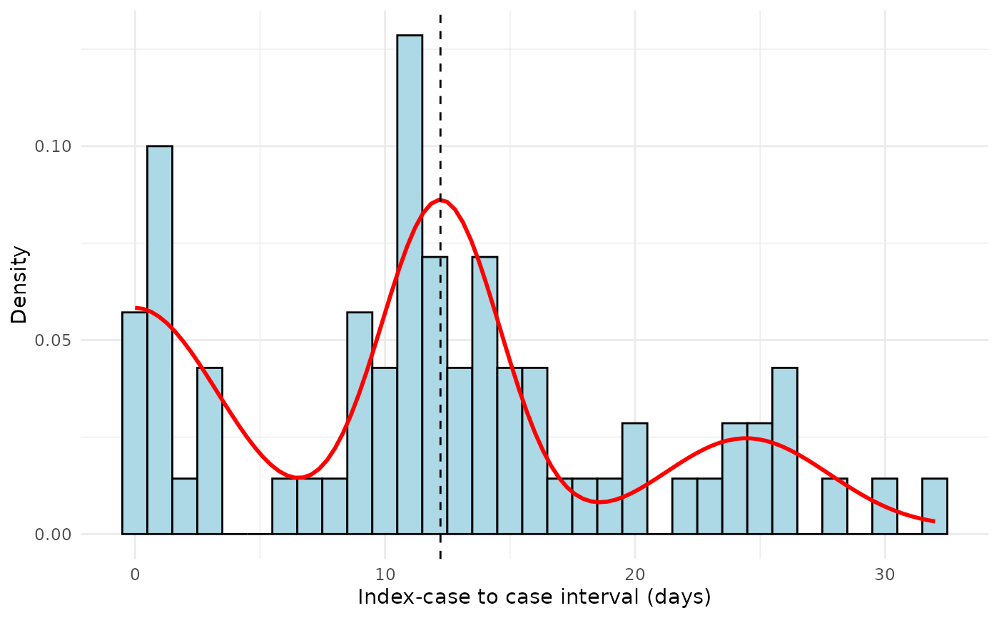
# 4 routes (default)
result <- si_estim(icc_data, n = 50)
plot_si_fit_result(result, icc_data, dist = "normal")
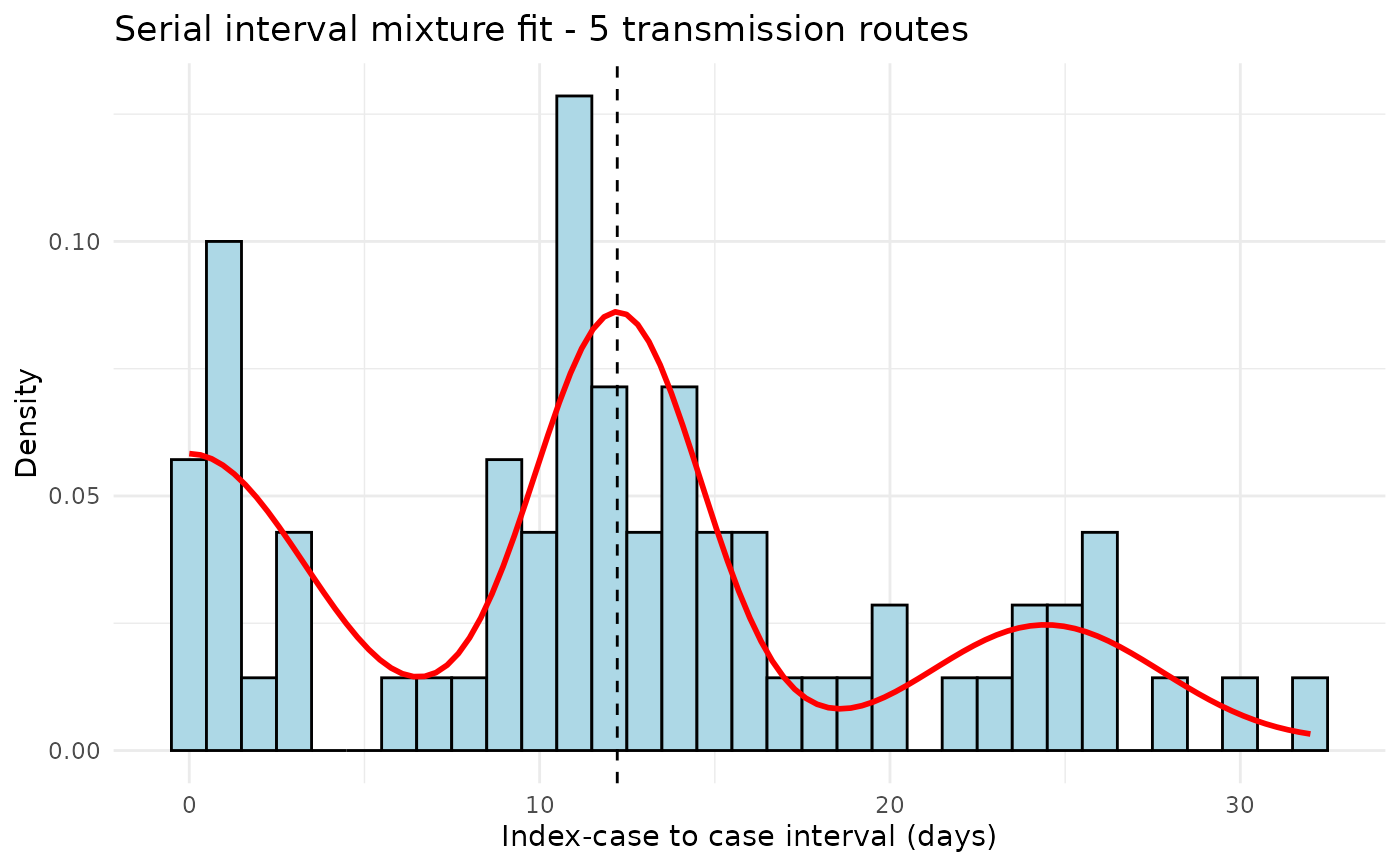
 # 5 routes
result5 <- si_estim(icc_data, n = 50, n_routes = 5)
plot_si_fit_result(result5, icc_data, dist = "normal")
# 5 routes
result5 <- si_estim(icc_data, n = 50, n_routes = 5)
plot_si_fit_result(result5, icc_data, dist = "normal")
 # }
# }