Code validation for Vink method
Kylie Ainslie
2026-06-04
Source:vignettes/articles/code_validation_for_Vink_method.Rmd
code_validation_for_Vink_method.RmdIntroduction
One of the motivations behind creating the mitey package
was to provide flexible, documented code for methods that can help
estimate epidemiological quantities of interest, such as the serial
interval, the time between the onset of symptoms in a primary case and
the onset of symptoms in a secondary case. In this article, we describe
a method developed by Vink
et al. 201418 to estimate
the mean and standard deviation of the serial interval distribution
using data on symptom onset times (see Methods for details). Further, we
demonstrate how to use mitey to apply this method to data,
and validate that we are able to produce the same estimates as those in
the original manuscript18.
Methods
The method proposed by Vink et al.18 was developed to estimate
characteristics of the serial interval distribution, namely the mean and
standard deviation, using data describing the the dates of symptom onset
for cases infected with a particular pathogen. The method involves
calculating the index case-to-case (ICC) interval for each person, where
the person with the greatest value for number of days since symptom
onset will be considered the index case. The rest of the individuals
will have an ICC interval calculated as the number of days between their
symptom onset date and the symptom onset date of the index case. The
method assumes that the ICC intervals can be split into different routes
of transmission: Co-Primary (CP), Primary-Secondary (PS),
Primary-Tertiary (PT), and Primary-Quaternary (PQ) based on the length
their ICC interval. The method constructs a likelihood function for ICC
intervals using a mixture model in which the mixture components are the
different transmission routes. Then, using the Expectation-Maximization
(EM) algorithm, the method iteratively calculates the probability that
an ICC interval falls into one of the four routes of transmission. The
method assumes an underlying Normal distribution for the serial interval
distribution, and has been extended to assume and an underlying Gamma
distribution. Both distributions can be specified in
si_estim using the dist = option.
Simulated Data
First we use simulated ICC intervals set to determine if we are able
to correctly estimate the mean and standard deviation of the simulated
serial interval using the si_estim function in the
mitey package. Here, we directly simulate the ICC intervals
based on their route of transmission. These simulated data are the same
as those provided in the supplemental material of Vink et al. The
specified mean serial interval hmu is 15 and the specified
standard deviation hsigma is 3. The weights for each route
of transmission are specified as hw1, hw2,
hw3, and hw4, respectively.
set.seed(1234)

N <- 10000; hmu<-15; hsigma<-3; hw1 <- 0.2; hw2 <- 0.5; hw3 <- 0.2; hw4 <- 0.1

CP <- fdrtool::rhalfnorm((hw1*N),theta=sqrt(pi/2)/(sqrt(2)*hsigma))
PS <- rnorm(hw2*N,mean=hmu,sd=hsigma)
PT <- rnorm(hw3*N,mean=2*hmu,sd=sqrt(2)*hsigma)
PQ <- rnorm(hw4*N,mean=3*hmu,sd=sqrt(3)*hsigma)

sim_data <- round(c(CP,PS,PT,PQ))
#> [1] 5 1 5 10 2 2 2 2 2 4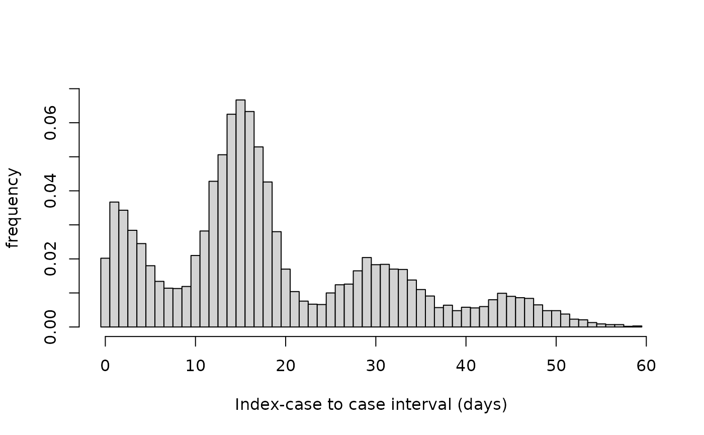
Figure 1. Histogram of index-case to case intervals (in days) for simulated data.
results<- si_estim(sim_data, dist = "normal")
results
#> $mean
#> [1] 15.03357
#>
#> $sd
#> [1] 2.786673
#>
#> $wts
#> [1] 2.100300e-01 4.823883e-01 6.706403e-09 2.003142e-01 2.304835e-15
#> [6] 1.072674e-01 9.057840e-22
#>
#> $converged
#> [1] TRUE
#>
#> $iterations
#> [1] 15
#>
#> $loglik
#> [1] -36757.5
#>
#> $n_restarts
#> [1] 1
#>
#> $n_routes
#> [1] 4
#>
#> $wind
#> [1] 1
The output of si_estim is a named list with elements
mean, sd, wts,
converged, iterations, loglik,
and n_restarts. The first three contain the estimated mean,
standard deviation, and weights of the serial interval distribution,
respectively. The additional fields provide convergence diagnostics:
converged indicates whether the EM algorithm converged
before reaching maximum iterations, iterations shows how
many iterations were performed, loglik provides the
log-likelihood for model comparison, and n_restarts
indicates how many random restarts were used. We see that using the
simulated data and assuming an underlying normal distribution, we obtain
estimates very close to the input values: a mean serial interval
estimate of 15.03 and a standard deviation of 2.79. We are also able to
recapture the input weights: hw1 = 0.21, hw2 = 0.48, hw3 = 0.2, hw4 =
0.11.
Using the plot_si_fit function, we can use the outputs
of si_estim to plot the fitted serial interval over the
symptom onset data.
plot_si_fit(
    dat = sim_data,
    mean = results$mean[1],
    sd = results$sd[1],
    weights = c(results$wts[1], results$wts[2] + results$wts[3],
                results$wts[4] + results$wts[5], results$wts[6] + results$wts[7]),
    dist = "normal"
  )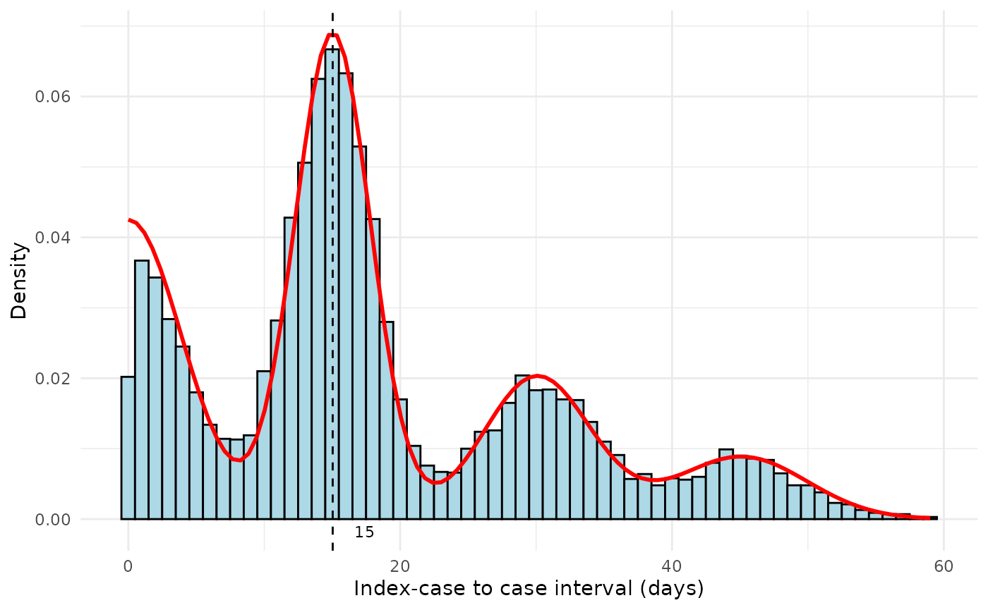
Figure 2. Fitted serial interval curves plotted over symptom onset data for simulated symptom onset data. Red line is the fitted serial interval curves assuming an underlying Normal distribution.
Historical Data
Next, we will estimate the mean serial interval using the method by
Vink et al.18 from different
historical data sets. The historical data are stored in
articles/validation_data.rds. The data set contains 5
columns:
-
Author: the first author of the published manuscript describing the data -
Year: the year the manuscript was published -
Pathogen: the pathogen of interest (e.g, influenza, measles) -
Country: the country in which the data were collected -
ICC_interval: the ICC intervals for each case described in the manuscript
#> # A tibble: 6 × 5
#>   Author Year  Pathogen Country ICC_interval
#>   <chr>  <chr> <chr>    <chr>          <dbl>
#> 1 Aaby   1990  Measles  Kenya              0
#> 2 Aaby   1990  Measles  Kenya              0
#> 3 Aaby   1990  Measles  Kenya              0
#> 4 Aaby   1990  Measles  Kenya              0
#> 5 Aaby   1990  Measles  Kenya              0
#> 6 Aaby   1990  Measles  Kenya              0
A useful feature of si_estim is that it can be applied
to multiple vectors of ICC intervals that are stored within a
long-format data frame using dplyr::summarise. An example
of how to do this is shown below using val_data. We first
select only the necessary columns, here Author, Pathogen, Country, and
ICC_interval. Then, we group the data, using group_by, by
Author, Pathogen, and Country, so that si_estim is applied
to the ICC intervals of only one study and one pathogen at a time.
Finally, we apply si_estim to each set of ICC intervals
using summarise. We can also specify the initial values
used to estimate the mean and standard deviation of the serial interval.
The default is the sample mean and sample standard deviation. The EM
algorithm is sensitive to the choice of initial value, so we will
specify the initial values from Table 2 in Vink et al. The initial
values are stored in articles/initial_values.rds. The
initial values for standard deviation are the minimum of the mean serial
interval divided by 2 or a random value drawn from uniform distribution
between 2 and 5. Finally, Due to the format of si_estim’s
output as a named list, we create new column for each estimate using
mutate and purrr:map_dbl.
initial_values <- readRDS("initial_values.rds")
val_data_w_init <- left_join(val_data, initial_values, by = "Pathogen")
results_historical <- val_data_w_init %>%
  group_by(Author, Pathogen, Country) %>%
  summarise(result = list(si_estim(.data$ICC_interval,
                                   init = c(first(.data$mean_si), first(.data$sd_si))
            ))) %>%
  mutate(
    mean = map_dbl(result, "mean"),
    sd = map_dbl(result, "sd"),
    wts = map(result, "wts")
  ) %>%
  select(-result)
The resulting output is a tibble with columns: Author, Pathogen,
Country, mean, sd, and wts. The mean and sd columns refer to the
estimates for the mean and standard deviation of the serial interval
distribution. The wts column refers to the weights for the different
transmission routes, and can be used as inputs when plotting the fitted
serial interval distribution using plot_si_fit. The weights
are stored as a list, so are not visible when printing the results, but
can be accessed using results_historical$wts.
#> # A tibble: 22 × 6
#> # Groups:   Author, Pathogen [20]
#>    Author    Pathogen               Country  mean    sd wts
#>    <chr>     <chr>                  <chr>   <dbl> <dbl> <list>
#>  1 Aaby      Measles                Kenya    9.93  2.40 <dbl [7]>
#>  2 Aycock    Rubella                Unknown 18.3   1.97 <dbl [7]>
#>  3 Bailey    Measles                England 10.9   1.93 <dbl [7]>
#>  4 Cauchemez Influenza A(H1N1)pdm09 USA      2.08  1.24 <dbl [7]>
#>  5 Chapin    Measles                USA     11.9   2.56 <dbl [7]>
#>  6 Crowcroft RSV                    England  7.52  2.11 <dbl [7]>
#>  7 Fine      Measles                England 13.7   1.50 <dbl [7]>
#>  8 Fine      Measles                USA     13.8   2.55 <dbl [7]>
#>  9 Fine      Smallpox               Germany 16.7   3.28 <dbl [7]>
#> 10 Fine      Smallpox               Kosovo  17.3   1.90 <dbl [7]>
#> # ℹ 12 more rows
When comparing the estimates produced by si_estim and
the estimates presented in Vink et al., we see that si_estim
successfully recaptures the estimates of the original study (Table
1).
Vink et al. Estimates |
si_estim Estimates |
||||||
|---|---|---|---|---|---|---|---|
Author |
Year |
Pathogen |
Country |
Mean |
SD |
Mean |
SD |
Hahne1 |
2009 |
Influenza A(H1N1)pdm09 |
Netherlands |
1.7 |
1.2 |
1.7 |
1.2 |
Cauchemez2 |
2009 |
Influenza A(H1N1)pdm09 |
United States |
2.1 |
1.2 |
2.1 |
1.2 |
Savage3 |
2011 |
Influenza A(H1N1)pdm09 |
Canada |
2.8 |
0.8 |
2.8 |
0.8 |
Papenburg4 |
2010 |
Influenza A(H1N1)pdm09 |
Canada |
2.9 |
1.2 |
2.9 |
1.2 |
France5 |
2010 |
Influenza A(H1N1)pdm09 |
United States |
3.0 |
0.9 |
3.0 |
0.9 |
Morgan6 |
2010 |
Influenza A(H1N1)pdm09 |
United States |
3.7 |
1.1 |
3.7 |
1.1 |
Viboud7 |
2004 |
Influenza A(H3N2) |
France |
2.2 |
0.8 |
2.2 |
0.8 |
Aaby8 |
1990 |
Measles |
Kenya |
9.9 |
2.4 |
9.9 |
2.4 |
Bailey9 |
1954 |
Measles |
England |
10.9 |
1.9 |
10.9 |
1.9 |
Simpson10 |
1952 |
Measles |
England |
10.9 |
2.0 |
10.9 |
2.0 |
Chapin11 |
1925 |
Measles |
United States |
11.9 |
2.6 |
11.9 |
2.6 |
Fine12 |
2003 |
Measles |
England |
13.7 |
1.5 |
13.7 |
1.5 |
Fine12 |
2003 |
Measles |
United States |
13.8 |
2.5 |
13.8 |
2.5 |
Simpson10 |
1952 |
Mumps |
England |
18.0 |
3.5 |
18.0 |
3.5 |
de Greeff13 |
2010 |
Pertussis |
Netherlands |
22.8 |
6.5 |
22.8 |
6.5 |
Crowcroft14 |
2008 |
RSV |
England |
7.5 |
2.1 |
7.5 |
2.1 |
Aycock15 |
1946 |
Rubella |
Unknown |
18.3 |
2.0 |
18.3 |
2.0 |
Fine12 |
2003 |
Smallpox |
Germany |
16.7 |
3.3 |
16.7 |
3.3 |
Fine12 |
2003 |
Smallpox |
Kosovo |
17.3 |
1.9 |
17.3 |
1.9 |
Vally16 |
2007 |
Varicella |
Australia |
13.1 |
2.2 |
13.1 |
2.2 |
Simpson10 |
1952 |
Varicella |
England |
14.1 |
2.4 |
14.1 |
2.4 |
Lai17 |
2011 |
Varicella |
Taiwan |
14.2 |
1.3 |
14.2 |
1.3 |
As with si_estim, the plotting function
plot_si_fit can be applied to numerous vectors of ICC
intervals using purrr:group_map. The results outputted from
si_estim cannot be used directly and must be merged with
the original ICC interval data. We will call this new data frame
df_merged and it should contain column(s) identifying the
study from which the ICC intervals correspond, as well as the mean,
standard deviation, and weights outputted from
si_estim.
#> # A tibble: 10 × 13
#>    Author Pathogen Country ICC_interval  mean    sd weight_1 weight_2  weight_3
#>    <chr>  <chr>    <chr>          <dbl> <dbl> <dbl>    <dbl>    <dbl>     <dbl>
#>  1 Aaby   Measles  Kenya              0  9.93  2.40    0.364    0.512 0.0000106
#>  2 Aaby   Measles  Kenya              0  9.93  2.40    0.364    0.512 0.0000106
#>  3 Aaby   Measles  Kenya              0  9.93  2.40    0.364    0.512 0.0000106
#>  4 Aaby   Measles  Kenya              0  9.93  2.40    0.364    0.512 0.0000106
#>  5 Aaby   Measles  Kenya              0  9.93  2.40    0.364    0.512 0.0000106
#>  6 Aaby   Measles  Kenya              0  9.93  2.40    0.364    0.512 0.0000106
#>  7 Aaby   Measles  Kenya              0  9.93  2.40    0.364    0.512 0.0000106
#>  8 Aaby   Measles  Kenya              0  9.93  2.40    0.364    0.512 0.0000106
#>  9 Aaby   Measles  Kenya              0  9.93  2.40    0.364    0.512 0.0000106
#> 10 Aaby   Measles  Kenya              0  9.93  2.40    0.364    0.512 0.0000106
#> # ℹ 4 more variables: weight_4 <dbl>, weight_5 <dbl>, weight_6 <dbl>,
#> #   weight_7 <dbl>
# Apply the plot_si_fit function by study
plots <- df_merged %>%
  group_by(Author, Pathogen, Country) %>%
  group_map(~ plot_si_fit(
    dat = .x$ICC_interval,
    mean = .x$mean[1],
    sd = .x$sd[1],
    weights = c(.x$weight_1[1], .x$weight_2[1] + .x$weight_3[1],
                .x$weight_4[1] + .x$weight_5[1], .x$weight_6[1] + .x$weight_7[1]),
    dist = "normal"
  ))

# Annotate plots with study names and labels
# Find the order of the groups
group_order <- df_merged %>%
  group_by(Author, Pathogen, Country) %>%
  group_keys()

labeled_plots <- lapply(seq_along(plots), function(i) {
  plots[[i]] +
    ggtitle(paste(group_order[i,1], group_order[i,2], group_order[i,3])) +
    theme(plot.title = element_text(size = 8, hjust = 0.5),
          axis.title.x = element_text(size = 8))
})

# Combine plots into a multi-pane figure
final_plot <- plot_grid(
  plotlist = labeled_plots[sample(1:22, 8)], # select studies to display randomly
  labels = "AUTO",      # Automatically adds labels (A, B, C, etc.)
  label_size = 12,      # Size of the labels
  ncol = 4              # Number of columns; adjust as needed
)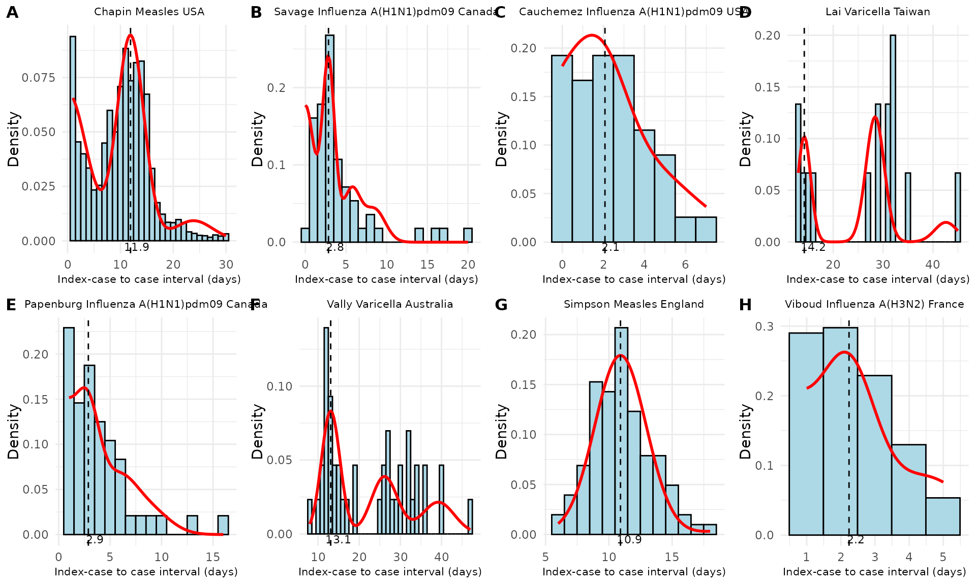
Figure 3. Fitted serial interval curves plotted over symptom onset data for a random sample of the historical data studies from Table 1. Red line is the fitted serial interval curves assuming an underlying Normal distribution.
Discussion
Here, we demonstrate how to use the mitey package to
estimate characteristics of the serial interval distribution by applying
a method developed by Vink et al. to commonly available symptom onset
data. We show that we are able to reproduce the estimates of the mean
and standard deviation of the serial interval distribution from the
original study when applying the method to numerous historical data sets
for a variety of pathogens.