Estimation of the epidemiological characteristics of scabies

Affiliations

Centre for Infectious Disease Control, National Institute for Public Health and the Environment (RIVM), Bilthoven, the Netherlands
School of Public Health, University of Hong Kong, Hong Kong SAR, China
Nivel, Utrecht, the Netherlands
Department of Biomedical Data Sciences, Leiden University Medical Center, Leiden, the Netherlands

This manuscript has not been peer-reviewed.

Abstract

Introduction: Scabies is a contagious skin disease caused by the infestation of the skin by the Sarcopes scabiei mite, causing an itchy rash. Scabies affects over 400 million people annually worldwide, and a rise in scabies cases has been observed in recent years throughout Western Europe. Despite the large number of people infected with scabies annually, some fundamental epidemiological characteristics of scabies infections have not been described.

Methods: In this work we use publicly available data on date of symptom onset during scabies outbreaks to determine the mean serial interval, time between symptom onset in an infector and symptom onset in an infectee, of scabies infection. We also use weekly numbers of persons consulting for scabies in primary care from sentinel surveillance in the Netherlands from 2011-2023 to determine quantities related to the spread of scabies over time, namely, the time-varying reproduction number, growth rate, and basic reproduction number.

Results: We found that there was considerable heterogeneity in estimates of the serial interval from different data sources, with mean serial interval estimates ranging from 98.4 days to 167.3 days. We estimated a pooled mean serial interval of 123.24 days (95% credible interval: 91.44, 153.41 days). An analysis of annual incidence of scabies per 1000 people in the Netherlands resulted in an estimated annual growth rate of 0.25 cases per 1000 people per year. Using the estimated growth rate and mean and standard deviation of the serial interval distribution we estimated the basic reproduction number, $R_0 = 1.09$ . When looking at scabies incidence over may years in the Netherlands, we saw yearly waves of infections, with the amplitude of incidence gradually increasing over time. We estimated the time-varying reproduction number by time of diagnosis and found that $R_t$ peaked for cases diagnosed in August.

Discussion: This study offers new insights into scabies transmission dynamics and suggests that additional interventions with limited efficacy that could prevent 8% of secondary infections would suffice to bring the reproduction number to below one. This may be achieved by increasing public awareness and targeted measures. These strategies may be effective in similar European settings. Our findings also underscore the need for precise data on scabies transmission, which could improve model accuracy for control strategies. Future research should focus on detailed characterization of scabies’ natural history to enhance intervention modeling and better inform containment efforts.

Introduction

Scabies is classified as a neglected tropical disease caused by infestation of the skin with a microscopic mite (Sarcoptes scabiei)¹. Symptoms are characterized by itchiness and rash at the site of infestation. Scabies affects around 400 million people per year, and accounts for a large proportion of skin disease in many low- and middle-income countries¹, particularly in tropical regions such as Asia, South America, and Oceania². Historically, scabies infections were a common affliction in Europe in the late 1800s and early 1900s with incidence peaking in 1918 and 1945^3,4. After the end of World War II, scabies incidence in Europe fell and remained low for decades^3–5. However, a rise in scabies cases has been observed through out Europe in recent years^6–11, which may increase the burden on healthcare systems due to scabies if the rising trend continues.

The global disease burden of scabies, expressed in disability-adjusted life years (DALY), is low compared to other infectious diseases. A 2017 study found that scabies was responsible for only 0.21% of DALYs from all conditions studied worldwide². However, areas with high scabies prevalence have been shown to have high disease burden of scabies partially due to secondary infections which can lead to severe outcomes². Additionally, there is no simple diagnostic self-test for scabies, so diagnosis relies on clinical assessment¹², which can increase the workload of general practitioners (GPs) during periods of high scabies incidence. Furthermore, individuals infected with scabies can suffer from stigma, discrimination and distress^12,13 in addition to the physical manifestations of the disease, making them less likely to seek medical care and further promoting transmission¹⁴. Research has also shown that scabies can have economic implications for both the patients and the healthcare system due to ineffective and long duration of treatment¹².

Despite the considerable burden scabies poses, little is known about the dynamics of scabies transmission, such as the generation time (time between infection of an index case and a secondary case), serial interval (the time from onset of symptoms in an index case to the time of symptom onset in a secondary case), growth rate, and reproduction number (the average number of secondary cases resulting from one index case). A series of studies in the 1940s by Kenneth Mellanby and colleagues^15,16 form much of the basis of our current understanding of scabies transmission. Some important results from the experiments performed in the 1940s by Mellanby and colleagues include an estimation of the incubation period, or time to symptom onset, of 4-6 weeks for first infections and 24 hours for subsequent infections; the parasite rate, defined as the number of mature female mites per person, over time, which was shown to increase rapidly, peak around 100 days after infection, and then decline quickly; and the probability of transmission via a secondary object (e.g., bed sheets) is low and most transmission occurs from person-to-person contact¹⁵. However, these studies were performed using healthy volunteers, so may not be representative of scabies transmission dynamics in other populations.

In this work, we aim to estimate key epidemiological characteristics of scabies, such as the serial interval, growth rate, and reproduction number, to better describe scabies transmission dynamics. Specifically, we use time series of reported symptom onset dates of scabies outbreaks from the literature to estimate the mean serial interval of scabies. We also use data on the number of scabies diagnoses each week in the Netherlands to estimate time-varying reproduction number and annual growth rate. To our knowledge, this is the first study to estimate these quantities for scabies, and can provide critical information for the design of appropriate infection control policy.

Methods

Data Sources

To estimate the mean serial interval for scabies infections, we conducted a rapid literature search to identify papers with publicly available data on date of symptom onset for scabies outbreaks. We searched Google images using the terms “scabies” and “epidemic curve” to find papers that featured symptom onset data over time and found 8 papers. Papers were excluded if data on date of symptom onset was not available or we were not able to reconstruct the date of symptom onset time series from the paper. We further excluded studies whose data did not span a sufficiently long time window for secondary infections to occur. We defined “sufficiently long” as 100 days based on the average peak parasite rate described by Mellanby¹⁵. After excluding papers that did not meet our criteria, we included a total of 4 papers in our analysis.

In addition to publicly available data on date of scabies symptom onset, we used high resolution data on the number of consultations for scabies over time in the Netherlands¹⁷ to estimate the time-varying reproduction number and growth rate. Briefly, we used published numbers of weekly numbers of persons consulting for scabies (per 100,000 population) from 2011 to 2023 as diagnosed by general practitioners (GPs). Scabies is recorded by ICPC code S72¹⁸. These are collected real-time in the nationally representative Nivel Primary Care Database (Nivel-PCD) of electronic health records from GPs, hosted by Nivel, the Netherlands institute for health services research¹⁹. Scabies is not a notifiable disease in the Netherlands, thus information on trends in incidence of scabies cases can only be obtained from GP diagnoses and dispensation of scabicides. Individuals in institutions (e.g., care homes, prisons) usually have their own health care provider and are generally not taken into account in GP registrations.

Serial Interval

Using the dates of symptom onset for scabies cases from four different studies^20–23 of scabies outbreaks (Table 1), we estimated the mean and standard deviation of the serial interval distribution using the method proposed by Vink et al.²⁴. Briefly, uses a maximum likelihood approach to approximate the mean and standard deviation of the serial interval distribution from the index case-to-case (ICC) interval for each person. The person with the greatest value for number of days since symptom onset will be considered the index case. The rest of the individuals will have an ICC interval calculated as the number of days between their symptom onset and the index case. The Vink method then weights the likelihood of each ICC interval being consistent with four routes of transmissions: 1) co-primary, 2) primary-secondary (serial interval), 3) primary-tertiary, and 4) primary-quaternary. Finally, using the ICC intervals consistent with primary-secondary transmission, we obtain an approximation of the serial interval distribution. The method requires the specification of the underlying serial interval distribution, either Gaussian (Normal) or Gamma. Here, we assumed that serial interval distributions for scabies can be approximated by a Normal distribution. Since serial intervals can be negative, albeit with low probability, the use of a distribution on a continuous scale is appropriate. The Gamma distribution has a more flexible shape, but as it is only defined for positive values of the serial interval it can only be used when the probability of negative values is very low. We performed a sensitivity analysis in which we assume the serial intervals for scabies can be approximated by a Gamma distribution (see Appendix).

We used the brms package in R²⁵ to estimate the pooled mean serial interval. We used a Bayesian hierarchical random-effects model in which we assume that there is a typical distribution for serial intervals, from which an outbreak-specific mean serial interval is sampled²⁶. We specified the prior distribution for the pooled mean as a normal distribution with a mean of 100 days, based on Mellanby’s reports on parasite rate and a standard deviation of 50 days to make sure the prior is not very informative. We used a Cauchy(0,1) distribution for the between-study heterogeneity. We performed sensitivity analyses on our choices of prior distributions (see Appendix).

Growth Rate and Basic Reproduction Number ( $R_0$ )

We estimated the annual growth rate of scabies cases by fitting a generalized linear model (GLM) with a log link and a quasipoisson family to the annual cumulative incidence of scabies diagnoses per 1000 people from 2011 to 2023 in the Netherlands²⁷. This approach accounts for the overdispersion commonly observed in count data and allows for non-integer values in the data. The GLM with a log link assumes an exponential growth model, where the logarithm of the expected count of scabies cases is linearly related to time and assumes quasipoisson distributed errors.

Using the fitted quasipoisson model, we determined the projected incidence of scabies per 1000 people until 2033, assuming no interventions are implemented and that the growth rate remains constant. We calculated 95% prediction intervals for the predicted incidence using standard error values adjusted to takes into account the dispersion parameter derived from the model, ensuring that our estimates appropriately reflect the uncertainty in the predictions.

Using the estimated annual growth rate, we can estimate the basic reproduction number as $R_0 = \exp(r*T – (1/2) r^2 s^2)$ , where $r$ is the annual growth rate, $T$ is the mean generation time (in years), and $s^2$ is the variance of the generation time distribution²⁸. We assume that nearly everyone exposed has not been previously infected.

Time-varying Reproduction Number

To estimate time-varying case reproduction number, we first randomly assigned each scabies consultation a date of diagnosis in the week in which the consultation is reported. Since scabies is very hard to diagnose prior to symptom onset¹⁶, and scabies consultations are captured as part of sentinel surveillance based on GP consultations²⁷, we use the date of consultation rather than the date of symptom onset. Using the constructed daily time series of date of diagnosis, we applied the method proposed by Wallinga and Lipsitch (Eq. 4.1)²⁸ to estimate the time-varying daily case reproduction number. The case reproduction number is defined as the average number of new infections that an individual who becomes diagnosed at a particular time point will go on to cause²⁹, and is useful in retrospective analyses such as the one presented here. The method of Wallinga and Lipsitch estimates the time-varying case reproduction number by determining the likelihood of an event occurring for every pair of time points²⁸. The method requires the specification of the serial interval distribution. We assumed a normal serial interval distribution with mean 123.24 days and standard deviation 31.55 days, as estimated above. Due to unobserved onward cases at the end of the time series, we adjusted for right truncation by applying a correction factor that accounts for unobserved cases with longer serial intervals. This factor is calculated using the cumulative distribution function of the assumed serial interval distribution to estimate the probability that a case with symptom onset at time t could have been observed given the current time T, with the inverse of this probability used as a weight for adjustment²⁹. To obtain 95% confidence intervals on the daily case reproduction number, we generated 100 bootstrapped samples by resampling each case with replacement and reconstructing the incidence time series for each bootstrapped sample. Reproduction number estimates were then smoothed using a rolling average of 6 weeks.

Because we are using the serial interval distribution as an approximation of the generation interval, which is strictly positive, we performed a sensitivity analysis in which we assumed the serial interval distribution is Gamma distributed with the same mean and variance.

All analyses were performed in R 4.4.0³⁰. Additional R packages used in this work are cited in the Appendix.

Results

Serial Interval

We estimated the mean and standard deviation of the serial interval using the epidemic curves from each study assuming an underlying Normal distribution (Table 1). There was considerable variation in the estimates of mean serial interval between studies. The shortest estimated mean serial interval (98.4 days) was estimated from data from Ariza et al.²⁰ describing an outbreak of scabies in a kindergarten in Germany. The largest estimated mean serial interval (167.34 days) was estimated from data from Kaburi et al.²¹ from an outbreak in a preschool in Ghana. Using data from an outbreak of scabies in a care home in the Netherlands²² we obtained an estimated mean serial interval of 110.7 days. Finally, we obtained an estimated mean serial interval of 122.9 days from data from an outbreak of scabies in a fishing community in the Hoima District of Uganda²³. We assessed the fitted serial interval distribution visually by plotting the estimated densities over the epidemic curves (Figure 1).

We performed a sensitivity analysis in which we estimated the mean and standard deviation of the serial interval assuming an underlying Gamma distribution (Table S1 and Figure S1). We found that we obtained similar mean estimates as compared to assuming an underlying Normal distribution (albeit lower for most studies), but the estimated standard deviations were larger. Model fit was assessed visually by plotting the estimated densities over the epidemic curves (Figure S1) and we found that the Gamma distribution was a poorer fit of the data as compared to the normal distribution.

Study	Mean	Standard Deviation
Akunzirwe et al.	122.92	26.92
Ariza et al.	98.40	8.54
Kaburi et al.	167.34	9.72
Tjon-Kon-Fat et al	110.72	16.14

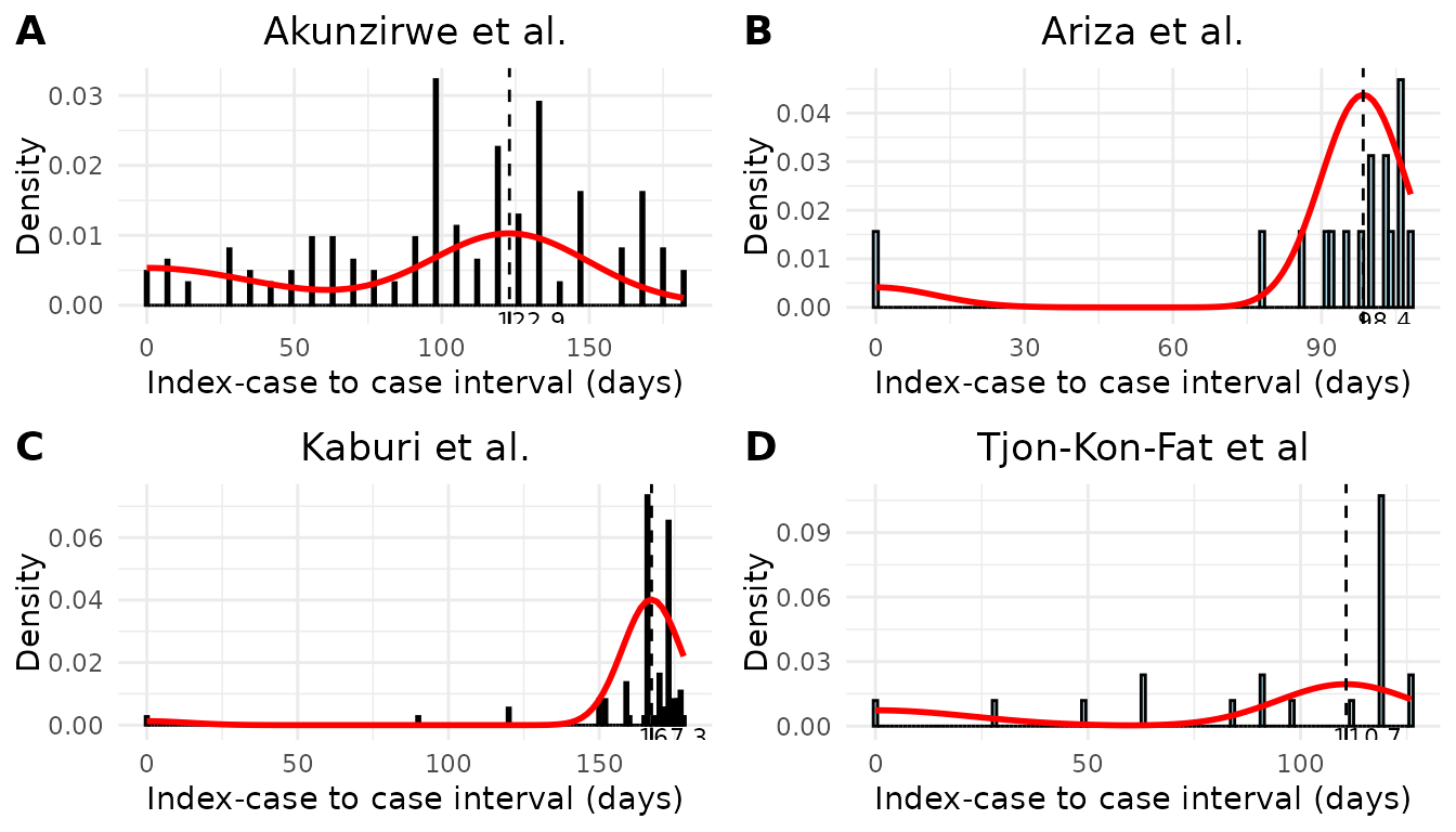
Figure 1. Model fit of the serial interval to index case–to–case (ICC) interval data. Each histogram shows the distribution of observed ICC intervals for scabies outbreaks described in A) Akunzirwe et al., B) Ariza et al., C) Kaburi et al., D) Tjon-Kon-Fat et al. The overlayed red line shows the estimated mixture density for each infection. The dashed vertical line indicates the mean serial interval. The value of the mean serial interval is shown to the right of the dashed line along the x-axis.

To obtain a pooled estimate of mean serial interval, we performed a meta-analysis using a Bayesian hierarchical framework in which we included random intercepts for each study. We estimated a pooled mean serial interval of 123.24 days (95% credible interval: 91.44, 153.41 days) (Figure 2). As we saw with the individual study estimates (Table 1), the analysis provided further evidence of substantial heterogeneity among studies due to a large value of the standard deviation of the random intercepts (31.55 days). The large variation in the mean serial interval estimates can be visualised by plotting the estimated distributions of each study’s serial interval shown in Figure 2). A normal distribution is assumed, and is parameterized by the estimated mean and standard deviation of serial interval for each study.

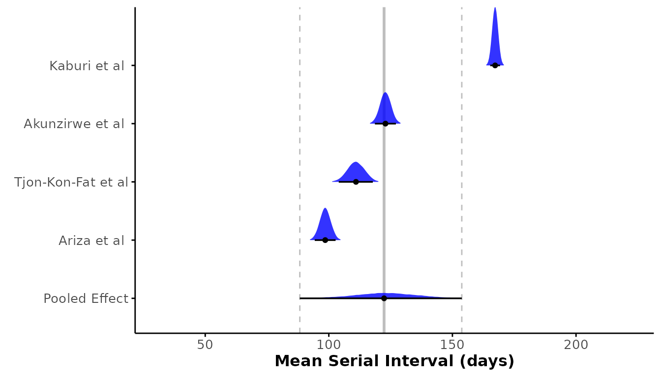
Figure 2. Forest plot of the estimated mean serial interval (in days) for individual studies and the pooled effect. The posterior distributions for each study are shown as density ridges, with the pooled effect displayed at the bottom. Black points and horizontal lines represent the posterior mean and corresponding 95% credible intervals for each study and the pooled estimate. The solid vertical gray line indicates the pooled effect estimate, while the dashed gray lines represent its 95% credible interval.

Growth Rate and Basic Reproduction Number ( $R_0$ )

We estimated the annual growth rate of scabies cases by fitting an exponential growth model to annual incidence of scabies per 1000 people from 2011 to 2023 in the Netherlands⁶. We estimated an annual growth rate of 0.25 (95% CI: 0.2, 0.3) . Using the previously estimated pooled mean serial interval (123.24 days or 0.34 years) and standard deviation of the serial interval (31.55 days or 0.09 years) as a proxy for the generation time, we estimated the basic reproduction number $R_0 =$ 1.09 (95% CI: 1.07, 1.11) . Using the fitted exponential growth model and the estimated growth rate, we then determined the projected annual incidence of scabies per 1000 people until 2033 if no interventions are implemented. We found that there could be a substantial increase in scabies incidence in the next 10 years in the Netherlands if no measures are taken to mitigate scabies spread (Figure 3).

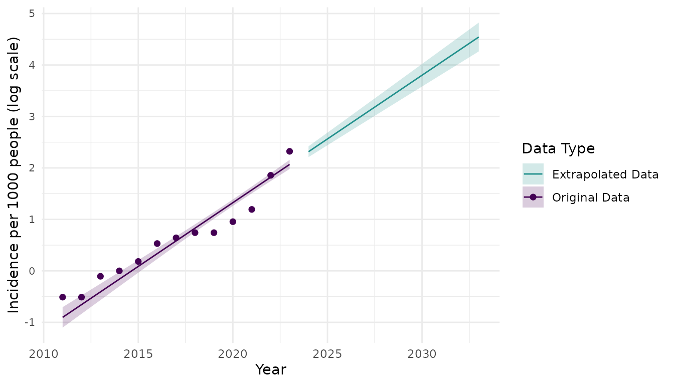
Figure 3. Annual scabies incidence per 1000 people from 2011 to 2023 (points) and then projected scabies indcidence per 1000 people for 2024 to 2033 (line) using an exponential growth model with annual growth rate of 0.25 (95% CI: 0.20, 0.30) cases per 1000 people. Shaded regions represent 95% prediction intervals for projected scabies incidence. The y-axis is displayed on the log-scale and represents the natural log of scabies incidence per 1000 people.

Time-varying Reproduction Number

To determine the pattern of scabies spread over time, particularly if the incidence of scabies infections displays a repeating temporal pattern (e.g., seasonal waves), we first plotted weekly incidence of scabies infections per 1000 people in The Netherlands from 2011 to 2023 (Figure 4). We observed approximate yearly peaks and troughs of incidence. Incidence was typically highest in October or November (however, in 2022, highest incidence occurred in December). There were additional rises in incidence in March-May (Figure S2) in most years. Cumulative incidence was typically lowest in the summer months June/July before rising again in August. We also observed that the amplitude of peak incidence gradually increasing over time. There were marked increases in peak incidence in 2022, 2023, and the beginning of 2024 (Figure 4). The observed patterns in scabies incidence indicate that there are approximately three generations of infections per year (Figure S2). For example, in 2023, one generation gets diagnosed in October, the next generation gets diagnosed in January the third generation gets diagnosed in May.

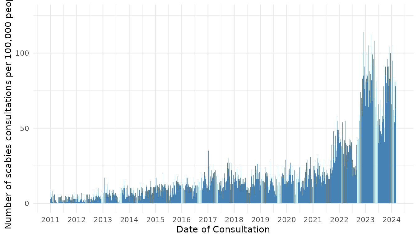
Figure 4. Number of scabies consultations per week per 100,000 people in the Netherlands by date of consultation.

Next, we estimated the time-varying case reproduction number of weekly scabies diagnoses (Figure 5). As with weekly incidence, we see temporal waves of transmission, with $R_t$ peaking in August. The time difference in peak incidence (October-January, Figure S2) versus peak reproduction number (June-September) can be explained by the long serial interval of scabies (123 days with a 31-day standard deviation). Therefore, infections generated by diagnosed cases in October-January are likely to manifest several months later, due to the long serial interval.

We performed a sensitivity analysis in which we estimated the time-varying reproduction number assuming an underlying gamma distribution for the serial interval with the same mean and standard deviation. We obtained similar estimates of $R_t$ as when we assumed the underlying serial interval distribution was a Normal distribution (Figure S3).

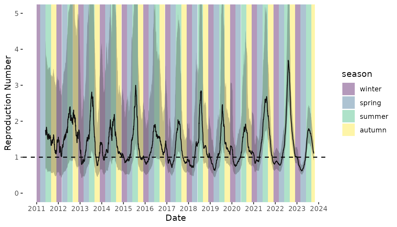
Figure 5. Time-varying case reproduction number of scabies transmission. Colored bands denote season. Winter = December 1 – February 28 (or 29 on leap year); Spring = March 1 – May 31; Summer = June 1 – August 31; Autumn = September 1 – November 31. Shaded region represents the 95% confidence envelope. Black horizontal dashed line indicates R = 1.

Discussion

In this work, we aimed to characterize scabies transmission dynamics by estimating key epidemiological parameters namely, the mean and standard deviation of the serial interval distribution, the basic reproduction number, the annual growth rate, and the time-varying reproduction number. Here, we provide some of the first estimates of the serial interval of scabies infection. We used symptom onset data from four previously published studies of scabies outbreaks and found that estimates of mean serial interval ranged from 98 days to 167 days. The large range in serial interval may be due to differences in study setting (school, nursing home, general population), contact patterns within those settings, and data quality. We performed a meta-analysis and obtained a pooled estimate of mean serial interval of 123 days. Our estimates of serial interval are considerably longer than the estimated incubation period (28-42 days) described by Mellanby¹⁵; however, our estimates of mean serial interval are of the same order of magnitude as the duration to reach peak scabies parasite rate (100 days since infection) plus the incubation period. Our pooled-estimate of mean serial interval should be used with caution. It was estimated by pooling data from studies in different populations, geographical locations, and settings, and using data on time of symptom onset. For more precise estimates of mean serial interval, future studies should collect information on transmission pairs.

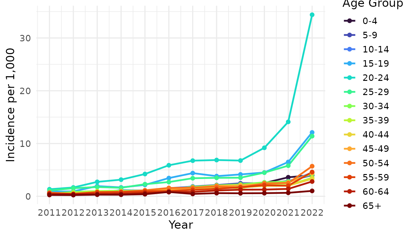
We observed seasonality in scabies transmission, finding that scabies incidence was highest in October and November, while the time-varying reproduction number peaked in the August. This pattern may be due to the long serial interval of scabies (123 days), whereby, the delayed onset of secondary cases shifts the peak in $R_t$ several months after the peak in incidence. The seasonal pattern in scabies incidence has been documented in other European countries^7–11,31 as well as the Western Pacific³². The seasonal pattern in scabies transmission can also be partially explained by the school calendar. Since scabies transmission has been shown to be driven by adolescents and young adults^6,7 (Figure S4), seasonal epidemics can be seeded at the start of the school year and peak in winter before reaching a trough in late spring and summer when the school year ends. Conversely, peak transmission could occur in summer when people are wearing less clothing; therefore, making skin-to-skin contact more probable, but cases are not detected until much later in the fall or winter.

Interestingly, in contrast to almost all notifiable infectious diseases, we found that the numbers of scabies cases increased during the COVID-19 pandemic (relative to years prior to the pandemic). Other infectious diseases, such as non-SARS-CoV-2 respiratory viruses, saw decreased incidence during the COVID-19 pandemic due to effective control measures³³ or underreporting and underdiagnosis⁶. The increase in scabies infections during the COVID-19 pandemic has also been observed in other countries, such as Ireland³⁴, Spain³⁵, Ethiopia³⁶, and Turkey³⁷. The increases in scabies infestations are likely due to increased indoor contact as a result of COVID-19 lockdowns and other control measures that restricted personal movement, such as curfews⁶, which often led to people staying overnight. With more time indoors, members of households share space for long periods, which may increase the risk of transmitting the scabies mites through direct contact or by fomites^34,35. Another explanation for an increase in scabies incidence in the Netherlands is the increased media coverage on scabies since 2021, which may have resulted in more scabies awareness and diagnoses than previous years.

Our study has several limitations. First, when estimating the serial interval and reproduction number, we assume that each infection is a person’s first infection. The time to symptom onset after infection (incubation period) has been described as 4-6 weeks for a person’s first infection, but only 24 hours for subsequent infections¹⁵. If a significant portion of individuals were experiencing a post-primary infection, then the estimated mean serial interval would likely be overestimated. Therefore, our estimates should be considered upper bounds of the average serial interval.

Second, when estimating the time-varying reproduction number, we used the pooled mean and standard deviation of the serial interval from the meta-analysis across studies of scabies epidemics. These studies varied in setting, geographic location, and study population, and the individual estimates of mean serial interval varied considerably across studies. It is possible that using the pooled mean and standard deviation from the meta-analysis does not represent the true mean serial interval among the Dutch population; however, no other estimates exist.

Third, to estimate the time-varying reproduction number we used data on date of scabies consultations. This data is only a proxy for true disease incidence data as the same person may have a consultation with their GP multiple times for the same infection. This may cause an overestimation of number of infections per week. We also assume that date of symptom onset is consistent with date of consultation (and subsequent scabies diagnosis). Since we do not know the delay between infection and consultation/diagnosis, we cannot precisely pinpoint the time that most transmission events occur. In a study of a scabies outbreak in a German school, the index case was not diagnosed for approximately 3 months following symptom onset²⁰. Similarly, in an outbreak analysis of a scabies outbreak in a preschool in Ghana, the likely primary case was not diagnosed for 10 weeks following symptom onset²¹. This delay in diagnosis can be due to the fact that scabies symptoms are not unique to scabies (itching, rash) or are misdiagnosed at first. While correcting for the delay between symptom onset and diagnosis of scabies cases would improve estimates of the time-varying reproduction number based on time of infection, this information is not routinely collected making correction for this delay difficult.

Our study highlights import areas for future research, namely, a) collecting data on scabies transmissions pairs to estimate the serial interval; b) characterizing the delay between symptom onset and GP consultation/diagnosis to correct estimates of the time-varying reproduction number estimated using GP consultations data; and c) reproducing estimates of the incubation period for scabies. The only estimate of the incubation period for scabies is the range provided by Mellanby of 4-6 weeks¹⁵. There is no data in the original study or in the literature to support this estimate or provide a point estimate with confidence bounds. Future research should aim to reproduce the original incubation period estimates and obtain more precise information on the incubation period of scabies infection.

Scabies continues to be a problem globally and better understanding of the epidemiological characteristics that govern scabies transmission can help containment efforts. We estimated that, in the Netherlands, $R_0=1.09$ , which is just above one. The required control effort to prevent the epidemic from growing is to prevent $(1-1/R_0) * 100\% = 8\%$ of all secondary infections. This reduction in secondary infections can be achieved with additional measures even if these have a low efficacy. Since 2023, the Dutch National Institute for Public Health and the Environment (RIVM) has published educational videos on their website as part of their Scabies Campaign (schurftcampagne)³⁸ to better inform the public about scabies infections, particularly young adults. While this campaign is too recent to show an impact on the results presented here, it may lead to a reduction in scabies infections in future. Additional interventions could include mass drug administration in large at risk groups, requiring a scabies check for university students prior to the school year, or informing GPs about the higher risk of scabies in certain groups to more quickly diagnose patients with symptoms consistent with a scabies infestation. While these strategies may not be effective in all locations where scabies is prevalent, they may help curb scabies infections in other European countries that have similar populations and scabies prevalence to the Netherlands.

In conclusion, this study has provided some of the first estimates of the epidemiological parameters governing scabies transmission. As evidence continues to suggest that scabies is a growing problem in European countries and remains a large problem elsewhere, the estimates provided here can help determine required control efforts to curb scabies epidemics. For example, the estimated epidemiological quantities can be used to parameterize mathematical models of scabies spread to determine the projected impact of different control measures. Prior mathematical modelling of scabies transmission have had to rely on the work of Mellanby¹⁵ for model parameterization^39–41. This work has also highlighted that very little is known about the transmission dynamics of scabies. Future work should focus on obtaining more precise information on the natural history of scabies infections to improve estimates of the underlying quantities that govern scabies spread.

Data Availability

All code, data, and scripts which reproduce the results of this paper can be found at https://github.com/kylieainslie/mitey.

Funding Statement

The study was financed by the Netherlands Ministry of Health, Welfare and Sport.

Role of the funding source

The funders of the study had no role in study design, data collection, data analysis, data interpretation, or writing of the report.

References

Control of Neglected Tropical Diseases (NTD). Report of the First WHO Global Meeting on Skin-Related Neglected Tropical Diseases: Geneva, Switzerland, 27–31 March 2023. (2024).

Karimkhani, C. et al. The global burden of scabies: A cross-sectional analysis from the global burden of disease study 2015. Lancet Infect. Dis. 17, 1247–1254 (2017).

Savin, J. A. Scabies in Edinburgh from 1815 to 2000. J. R. Soc. Med. 98, 124–129 (2005).

Christophersen, J. The epidemiology of scabies in Denmark, 1900 to 1975. Arch. Dermatol. 114, 747–750 (1978).

Downs, A. M., Harvey, I. & Kennedy, C. T. The epidemiology of head lice and scabies in the UK. Epidemiol. Infect. 122, 471–477 (1999).

Deursen, B. van et al. Increasing incidence of reported scabies infestations in the netherlands, 2011-2021. PLoS One 17, e0268865 (2022).

Reichert, F., Schulz, M., Mertens, E., Lachmann, R. & Aebischer, A. Reemergence of scabies driven by adolescents and young adults, germany, 2009-2018. Emerg. Infect. Dis. 27, 1693–1696 (2021).

Redondo-Bravo, L. et al. Scabies in spain? A comprehensive epidemiological picture. PLoS One 16, e0258780 (2021).

Lugović-Mihić, L. et al. An increasing scabies incidence in croatia: A call for coordinated action among dermatologists, physicians and epidemiologists. Zdr Varst 59, 264–272 (2020).

10.

Amato, E. et al. Increase of scabies infestations, norway, 2006 to 2018. Euro Surveill. 24, (2019).

11.

Donà, M. G. et al. Increasing trend in confirmed scabies cases in the only public dermatological institute of scientific research and care in italy. Eur. J. Dermatol. 33, 709–710 (2023).

12.

Cox, V., Fuller, L. C., Engelman, D., Steer, A. & Hay, R. J. Estimating the global burden of scabies: What else do we need? Br. J. Dermatol. 184, 237–242 (2021).

13.

White, A. V., Hoy, W. E. & McCredie, D. A. Childhood post-streptococcal glomerulonephritis as a risk factor for chronic renal disease in later life. Med. J. Aust. 174, 492–496 (2001).

14.

Mitjà, O. et al. Integrated control and management of neglected tropical skin diseases. PLoS Negl. Trop. Dis. 11, e0005136 (2017).

15.

Mellanby, K. The development of symptoms, parasitic infection and immunity in human scabies. Parasitology 35, 197–206 (1944).

16.

Mellanby, K. Scabies. (EW Classey, Faringdon, England, 1972).

17.

M. Hooiveld, Y. W. A. F. S. Surveillance of infectious diseases based on electronic medical records in primary care in 2016. in State of infectious diseases in the netherlands 2016 (eds. Gier, J. W. D. de, D. R. E. Nijsten & S. J. M. Hahné, B.) 25–30 (Rijksinstituut voor Volksgezondheid en Milieu (RIVM), Bilthoven, 2017).

18.

World Organization of National Colleges of Physicians. ICPC. International Classification of Primary Care. (Oxford University Press, Oxford, England, 1987).

19.

Hasselaar, J. Nivel primary care database.

20.

Ariza, L. et al. Investigation of a scabies outbreak in a kindergarten in constance, germany. Eur. J. Clin. Microbiol. Infect. Dis. 32, 373–380 (2013).

21.

Kaburi, B. B. et al. Outbreak of scabies among preschool children, accra, ghana, 2017. BMC Public Health 19, 746 (2019).

22.

Tjon-Kon-Fat, R. et al. Short report: The potential of PCR on skin flakes from bed linens for diagnosis of scabies in an outbreak. PLoS Negl. Trop. Dis. 15, e0009485 (2021).

23.

Akunzirwe, R. et al. An outbreak of scabies in a fishing community in hoima district, uganda, February−June, 2022. Research Square (2023).

24.

Vink, M. A., Bootsma, M. C. J. & Wallinga, J. Serial intervals of respiratory infectious diseases: A systematic review and analysis. Am. J. Epidemiol. 180, 865–875 (2014).

25.

Bürkner, P.-C. Brms: An R package for bayesian multilevel models using stan. J. Stat. Softw. 80, 1–28 (2017).

26.

Harrer, M., Cuijpers, P., Furukawa, T. A. & Ebert, D. D. Chapter 13 bayesian Meta-Analysis.

27.

NIVEL. Cijfers ziekten per week in nederland.

28.

Wallinga, J. & Lipsitch, M. How generation intervals shape the relationship between growth rates and reproductive numbers. Proc. Biol. Sci. 274, 599–604 (2007).

29.

Gostic, K. M. et al. Practical considerations for measuring the effective reproductive number, rt. PLoS Comput. Biol. 16, e1008409 (2020).

30.

R Core Team. R: A Language and Environment for Statistical Computing. (R Foundation for Statistical Computing, Vienna, Austria, 2019).

31.

Korycinska, J., Dzika, E. & Kloch, M. Epidemiology of scabies in relation to socio-economic and selected climatic factors in north-east poland. Ann. Agric. Environ. Med. 27, 374–378 (2020).

32.

Ducrot, Y.-M. et al. Scabies incidence and association with skin and soft tissue infection in loyalty islands province, new caledonia: A 15-year retrospective observational study using electronic health records. PLoS Negl. Trop. Dis. 16, e0010717 (2022).

33.

Chow, E. J., Uyeki, T. M. & Chu, H. Y. The effects of the COVID-19 pandemic on community respiratory virus activity. Nat. Rev. Microbiol. 21, 195–210 (2023).

34.

Griffin, L. R., Pender, E. K., Laing, M. E. & Markham, T. Unexpected consequences of SARS-CoV-2 pandemic: Scabies infestation. Clin. Exp. Dermatol. 47, 1196–1197 (2022).

35.

Martínez-Pallás, I., Aldea-Manrique, B., Ramírez-Lluch, M., Manuel Vinuesa-Hernando, J. & Ara-Martín, M. Scabies outbreak during home confinement due to the SARS-CoV-2 pandemic. J. Eur. Acad. Dermatol. Venereol. 34, e781–e783 (2020).

36.

Asgedom, A. A., Debesay, M. H., Ugwu, C. L. J. & Woldegerima, W. A. Detecting spatial clusters of human scabies in tigray, ethiopia from 2018 to 2023. BMC Infect. Dis. 24, 1148 (2024).

37.

Akaslan, T. Ç., Mert, Ö. & Su Küçük, Ö. Scabies increase during the COVID-19 pandemic: Should we change our treatment strategy during the pandemic? Ann. Parasitol. 68, 35–38 (2022).

38.

RIVM. Video’s over schurft.

39.

Kinyanjui, T. et al. Scabies in residential care homes: Modelling, inference and interventions for well-connected population sub-units. PLoS Comput. Biol. 14, e1006046 (2018).

40.

Lydeamore, M. J. et al. A biological model of scabies infection dynamics and treatment informs mass drug administration strategies to increase the likelihood of elimination. Math. Biosci. 309, 163–173 (2019).

41.

Tellioglu, N. et al. Modelling mass drug administration strategies for reducing scabies burden in monrovia, liberia. Epidemiol. Infect. 151, e153 (2023).

42.

Klaus, B. & Strimmer., K. Fdrtool: Estimation of (Local) False Discovery Rates and Higher Criticism. (2021).

43.

Wilke, C. O. Cowplot: Streamlined Plot Theme and Plot Annotations for ’Ggplot2’. (2024).

44.

Wickham, H., Hester, J., Chang, W. & Bryan, J. Devtools: Tools to Make Developing r Packages Easier. (2022).

45.

Wickham, H., François, R., Henry, L., Müller, K. & Vaughan, D. Dplyr: A Grammar of Data Manipulation. (2023).

46.

Wickham, H., Bryan, J., Barrett, M. & Teucher, A. Usethis: Automate Package and Project Setup. (2024).

47.

Wickham, H. Ggplot2: Elegant Graphics for Data Analysis. (Springer-Verlag New York, 2016).

48.

Gohel, D. & Skintzos, P. Flextable: Functions for Tabular Reporting. (2024).

49.

Yasumoto, A. ftExtra: Extensions for ’Flextable’. (2024).

50.

Schauberger, P. & Walker, A. Openxlsx: Read, Write and Edit Xlsx Files. (2023).

51.

Wickham, H. et al. Welcome to the tidyverse. Journal of Open Source Software 4, 1686 (2019).

52.

Robinson, D., Hayes, A. & Couch, S. Broom: Convert Statistical Objects into Tidy Tibbles. (2024).

53.

Garnier et al. viridis(Lite) - Colorblind-Friendly Color Maps for r. (2024). doi:10.5281/zenodo.4679423.

54.

Gohel, D. & Moog, S. Officer: Manipulation of Microsoft Word and PowerPoint Documents. (2024).

55.

Kay, M. tidybayes: Tidy Data and Geoms for Bayesian Models. (2023). doi:10.5281/zenodo.1308151.

56.

Wilke, C. O. Ggridges: Ridgeline Plots in ’Ggplot2’. (2024).

57.

Hester, J. & Bryan, J. Glue: Interpreted String Literals. (2024).

58.

Zeileis, A. & Grothendieck, G. Zoo: S3 infrastructure for regular and irregular time series. Journal of Statistical Software 14, 1–27 (2005).

59.

Wickham, H. Stringr: Simple, Consistent Wrappers for Common String Operations. (2023).

60.

Wickham, H. Forcats: Tools for Working with Categorical Variables (Factors). (2023).

61.

Harrell Jr, F. E. Hmisc: Harrell Miscellaneous. (2024).

Appendix

Sensitivity Analyses

Serial Interval

We performed a sensitivity analysis on the underlying distribution of serial interval. In the main analysis we assumed the serial interval was normally distributed. In the sensitivity analysis we assumed the serial interval was Gamma distributed. The estimated mean and standard deviation of serial interval for each study is shown in Table S1 . When assuming an underlying Gamma distribution, the standard deviations were higher than when assuming an underlying Normal distribution. We see from Figure S1 that the Gamma distribution does not fit the data well. It is possible that the Gamma distribution fits scabies data poorly due to the long incubation period of scabies and the possibility of negative serial intervals.

Study	Normal		Gamma
Study	Mean	SD	Mean	SD
Akunzirwe et al.	122.9239	26.920354	105.29254	92.61143
Ariza et al.	98.4000	8.542332	91.49460	113.66905
Kaburi et al.	167.3444	9.717630	164.68478	21.41681
Tjon-Kon-Fat et al	110.7157	16.138793	94.30272	107.28626
SD = standard deviation

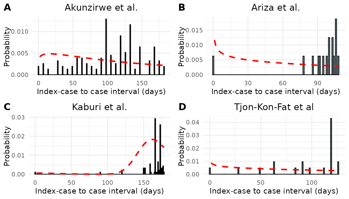
Figure S1. Epidemic curves and estimated serial interval distributions from four scabies outbreaks. Red line indicates estimated serial interval density assuming an underlying gamma distribution.

We performed a sensitivity analysis in which we altered our choice of prior distribution for mean serial interval. In the main analysis we assumed a prior distribution of N(100,50). In the sensitivity analysis we assumed a prior distribution of N(50, 75) and N(150, 50). We obtained similar estimates of the pooled mean serial interval under the alternative prior distributions (Table S2).

Prior	Mean	Standard Deviation
N(100, 50)	123.24	31.55
N(50, 75)	120.87	32.22
N(150, 50)	127.15	31.73

Time-varying Reproduction Number

To see how incidence of scabies varied by month, we plotted the cumulative incidence of scabies cases per 1000 people in the Netherlands by month for each year between 2011 and 2023 (Figure S2).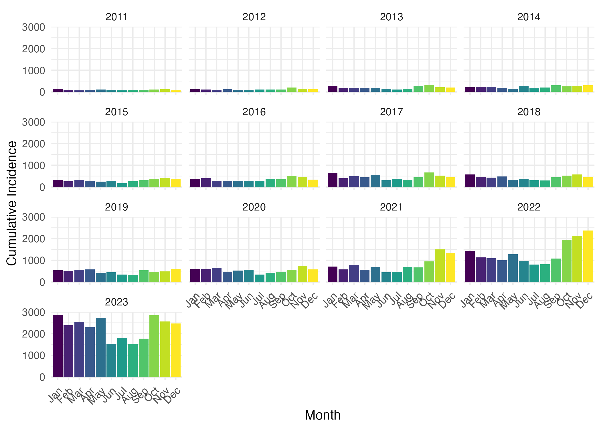

Figure S2. Cumulative consulatations for scabies per 100,000 people in the Netherlands by month and year.

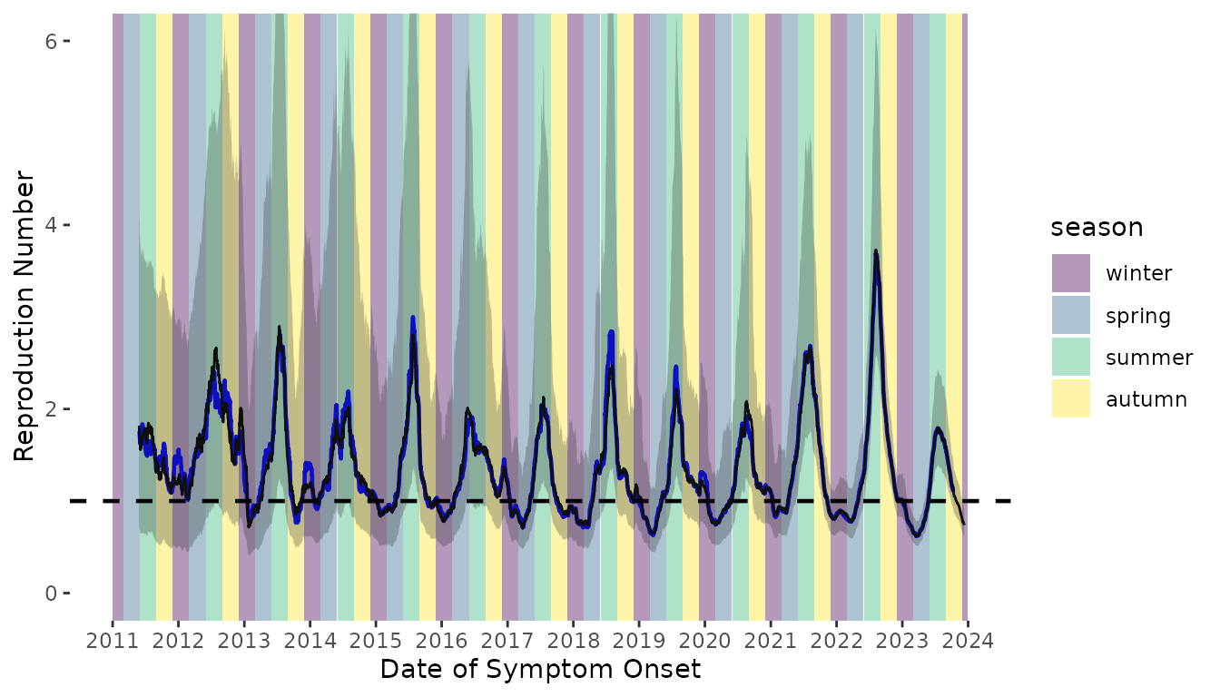
In the main analysis, when we estimate the time-varying reproduction number, we assume an underlying Normal distriubtion. However, because we are using the serial interval distribution as an approximation of the generation interval, which is strictly positive, we performed a sensitivity analysis in which we assumed the serial interval distribution is Gamma distributed with the same mean and variance (Figure S3).

Figure S3. Time-varying reproduction number of scabies transmission assuming a Gamma distributed serial interval distribution (black line). The time-varying reproduction number estimates assuming an underlying normal serial interval distribution are shown as the blue line. Colored bands denote season. Winter = December 1 – February 28 (or 29 on leap year); Spring = March 1 – May 31; Summer = June 1 – August 31; Autumn = September 1 – November 31.

Annual Incidence by Age Group

Figure S4. Annual scabies incidence per 1,000 people by age group in the Netherlands from 2011 to 2022.

Computing details

The additional R packages used in this work that have not previously been mentioned or cited in the main text are fdrtool⁴², cowplot⁴³, devtools⁴⁴, dplyr⁴⁵, usethis⁴⁶, ggplot2⁴⁷, flextable⁴⁸, ftExtra⁴⁹, openxlsx⁵⁰, tidyverse⁵¹, broom⁵², viridis⁵³, officer⁵⁴, tidybayes⁵⁵, ggridges⁵⁶, glue⁵⁷, zoo⁵⁸, stringr⁵⁹, forcats⁶⁰, Hmisc⁶¹.

References

bibliography: appendix_references.bib